Topological Autoencoders.

Preface

With this post I intend to familiarize the reader with Topological Autoencoders, a novel method for preserving topological properties of high-dimensional data in low-dimensional representations of autoencoders. While we are going to present this paper at ICML2020, this blog post should serve as a high-level, foremost visual, and easily digestible appetizer before reading the actual paper.

Motivation

Let’s consider a dataset of high-dimensional sphere manifolds (specifically, $100$-spheres), with one large sphere enclosing 10 smaller spheres. We are given noisy samples which are observed close to these manifolds.

We find that it is surprisingly hard to preserve the global structure of the data space, i.e. the nesting relationship of the spheres, in low dimensional representations.

When we train an autoencoder with a two dimensional bottleneck, the spheres are merely pulled apart and the global structure is lost (see below animation on the left). To address this, we propose a topological loss term which makes the autoencoder aware of the topological features in both the data space and the latent space, incentivizing the model to preserving the data space topology in the low dimensional representations (see below animation on the right)

Background

Topology - The study of connectivity

Two spaces are considered homeomorphic (which is a type of topological equivalence), if there exists a bijective, continuous, and invertible mapping between them, whereas the inverse is also continuous. For instance, a torus and a mug would be homeomorphic as they can be transformed into each other without tearing or cutting.

image source

One way to determine topological properties of a space is to determine its Betti numbers which represent its number of $d$-dimensional holes. For instance, $d=0$ refers to the number of connected components, $d=1$ to its tunnels, and $d=2$ to its voids). Consequently, the $2$-torus which can be elegantly described as the Cartesian product of two $1$-spheres, i.e., circles, shows the Betti numbers: $(1,2,1)$.

The application of topological methods to real-world data is referred to as Topological Data Analysis (TDA). One key challenge here is that we typically don’t observe manifolds directly but only sampled data points which may lie near manifolds (as visualized below, credits to @PseudoManifold).

torus manifold (above) versus point cloud of data points (below)

Given a point cloud of unconnected points, how can we detect properties like tunnels, voids etc which are captured with the above Betti numbers?

Calculating Betti Numbers

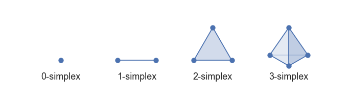
In simplicial homology, Betti numbers can be directly calculated from a simplicial complex. (Formally, the $i$-th Betti number refers to the rank of the $i$-th homology group of the simplicial complex). But what is a simplicial complex? To answer this, we first need to define simplices: A (combinatorial) $k$-simplex is the convex hull of $k + 1$ vertices.

image source

Using that, we can define a simplicial complex $\mathfrak{K}$ as a set of $k$-simplices (of potentially varying $k$) fulfilling two criteria:

1. every face of a simplex in $\mathfrak{K}$ is also in $\mathfrak{K}$.
2. any non-empty intersection of two simplices in $\mathfrak{K}$ is a face of both simplices.

Example:

image source

But how to arrive at a simplicial complex from a point cloud of data points? Which points should be connected? This is a non-trivial problem since adding or removing single points could change the Betti numbers of the resulting simplicial complex! This issue motivates persistent homology: using a varying threshold $\epsilon$, we can extract a nested sequence of simplicial complexes to extract topological features over varying scales (‘multi-scale Betti numbers’). This process of creating a nested sequences of complexes is refered to as filtration. For instance, by growing $\epsilon$-balls, we create a Vietoris-Rips (VR) complex.

During this filtration over $\epsilon$-scales, topological features (tunnels, voids etc.) are created and destroyed. As a standard way to capture this we enter both the creation scale $\epsilon_1$ ($x$-axis) and the destruction scale $\epsilon_2$ ($y$-axis) for each feature into a persistence diagram. It is generally assumed that topologically relevant features (corresponding to global structure) lead to off-diagonal entries whereas noisy features appear close to the diagonal in the persistence diagram. Below, we visualize a VR filtration for a given point cloud while we continuously fill the persistence diagram on the right.

Topological Autoencoders

Now that we have built some intuition about persistent homology calculations, let’s sketch our proposed method. We start with a deterministic autoencoder setup. On top of that, we compute a VR filtration both in the data space as well as in the latent space on the level of the minibatch. This means, that our considered point cloud consists of data points of one minibatch. The idea here is to extract topological descriptors from both spaces in order to derive a loss term which incentivizes the model to learn representations that preserve the data space topology.

To further ignite your curiosity, we flash here a set of challenges we had to address to get this method work smoothly:

1. How can we extract topological features of the data and latent space by means of a VR filtration on the minibatch-level?

2. Given the discrete nature of topological calculations, how can we construct a topological loss term in a way that it is differentiable such that the entire pipeline can be trained end-to-end with backpropagation?

3. How can we compare the persistence diagrams of the two spaces given that they may not show the same number of entries that also refer to different edges in the VR complex?

We address those problems in detail in our paper. In there, various experiments, evaluations as well as more visualizations are awaiting you, so feel free to have a look!

Finally, to give you a first glimpse of our results, below we depict $2D$ representations of the high-dimensional spheres dataset for various dimensionality reduction techniques.

PCA		t-SNE
UMAP		Isomap
AE		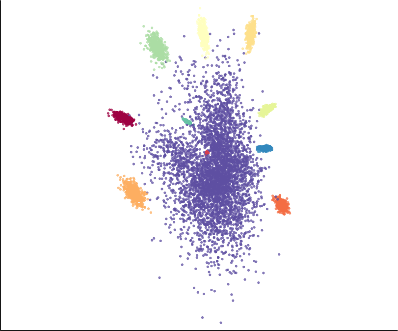TopoAE

We find that our proposed method, TopoAE, was the only one able to preserve the global structure of the dataset, i.e. the complex nesting relationship of the spheres. Interestingly, t-SNE partially preserved the nesting relationship -- but only on a localized level (the large sphere is not surrounding all smaller ones). As indicated, for more details, more datasets, and importantly, also for quantitative evaluations, please refer to our [paper](https://arxiv.org/abs/1906.00722).

Further pointers

• talk
• preprint
• code

Acknowledgments

First off, I would like to thank Max Horn (co-first author), Bastian Rieck (co-last author and TDA expert of this project), and Karsten Borgwardt (co-last author and my PhD advisor). Next, I would like to thank Christian Bock for fruitful discussions, as well as the entire MLCB lab for its support.
The animations of this post were created using the manim library, generously provided by 3Blue1Brown. The visualized persistence diagram was computed using the Aleph library, generously provided by @PseudoManifold.